Photo Geolocation with a Multi-Input Convolutional Neural Network

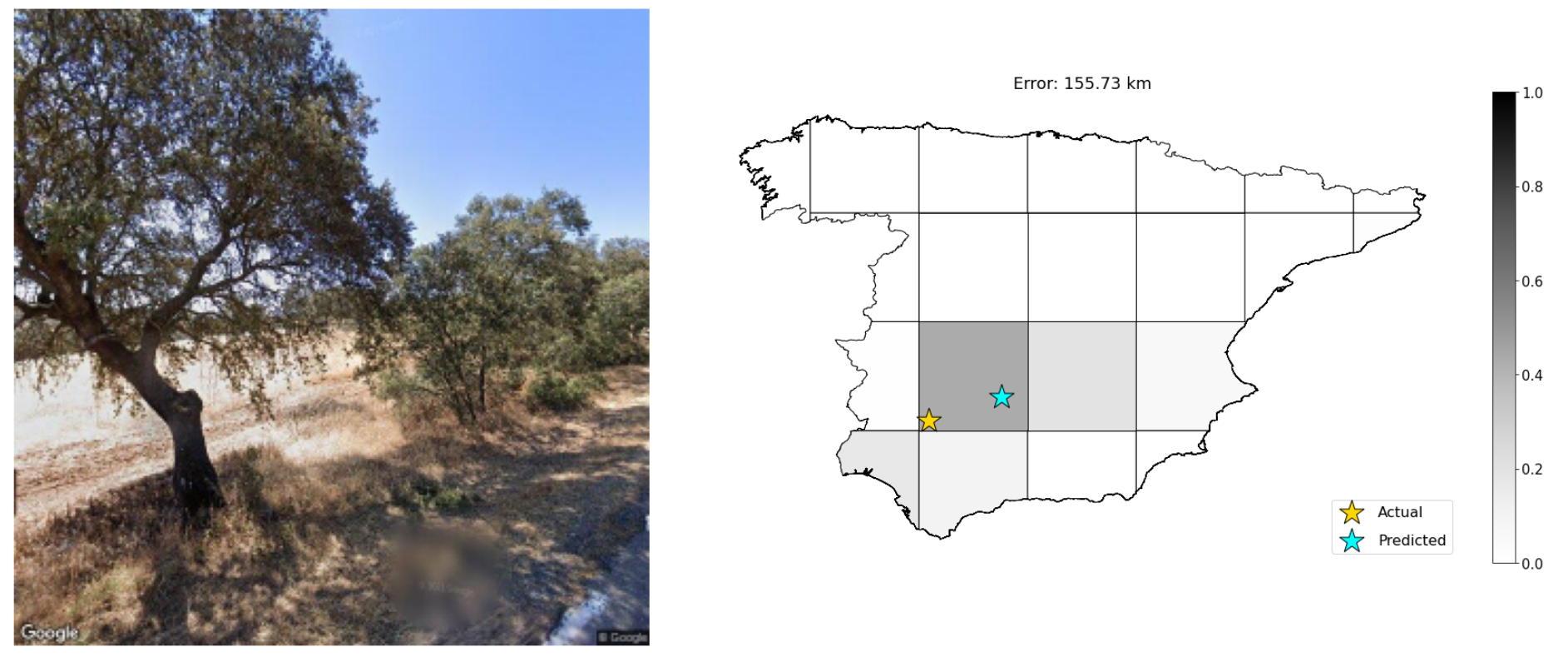
For my final project in CSC262: Computer Vision at Grinnell College, I addressed the problem of photo geolocation: the task of determining the location on Earth at which a given photo was taken based on its content. For the sake of feasibility (and also to add something new to existing literature that focuses on a global scale), my project considered photo geolocation in mainland Spain alone.

This project when through two stages. I provided an initial version at the end of the course to serve as my final project. In this version, the model’s output was a longitude and latitude value representing the predicted location at which the image was taken. Following my final presentation, my professor (Jerod Weinman) proposed that prediction could be improved by splitting mainland Spain into a grid layout and outputting a multinomial probability distribution with values representing the probability that an image was taken in a certain cell.

I did, in fact, implement these changes after completing the course. On this page, I will present results from the latter version. While it doesn’t change a whole lot, I should note that the GitHub repository here and paper here correspond to the former version. Much of the content of this page is copy-and-pasted from the aforementioned paper, but some details are left out (like a comparison between the final feature-based CNN model versus a simple feature-based model and a basic CNN). These can be found in the paper.

Abstract

Can we accurately predict the location at which an image was taken using the information provided by the image’s pixels? This question describes the problem of photo geolocation. Previous foundational research has approached the problem at the global scale using either classical features or convolutional networks. In this paper, I analyze images from a data set of a smaller scale, specifically the country of Spain. I adapt previously implemented photo geolocation techniques using either classical features or convolutional networks, and then I implement a model that incorporates both methodologies. I find that a convolutional network is a significant improvement over an approach that only considers classical features. Furthermore, incorporating classical features into a convolutional neural network along with an image input has a minor positive effect on performance. These findings suggest that classical features do not have significant utility in the problem of small-scale photo geolocation when convolutional neural networks are available as an option.

Introduction

Photo geolocation is described as the task of determining an input photo’s location using just the image’s content itself.¹ The photo geolocation problem is a familiar computer vision task due to the proof of concept provided by human example² and the value that a viable solution would hold. The accurate geotagging provided by a viable photo geolocation solution could be used for secondary computer vision tasks such as object recognition¹ and could even benefit response time for emergency aid.³

Notable past approaches to the photo geolocation problem include IM2GPS¹ and PlaNet.⁴ Both papers leveraged a vast global data set featuring both urban and rural photos - they differed in predictive model framework. While the authors of the IM2GPS paper employed feature descriptors to predict an image’s geolocation, the authors of the PlaNet paper instead depended upon a convolutional neural network for this task. Both approaches achieved state-of-the-art success at the time of their publishing.

In the context of prior literature, this project contributes a slightly different framework to the photo geolocation problem. Instead of a large-scale outlook, the analysis will be limited to the national level, specifically the country of Spain (mainland). The motivation for this choice is based upon the assumption that image variability increases over larger distances - identifying visual differences between north and south Spain should be a more difficult task than identifying visual differences between North America and South America. Thus, it is my intention to determine how well a photo geolocation model can perform at a smaller scale where geographic and biological variance is lower.

Furthermore, the model framework also differs from those of the IM2GPS and PlaNet studies. In this paper, I will combining aspects of both models by training a convolutional neural network that incorporates various global feature descriptors. While doing so, I will also explore the relative performance between both techniques (i.e. only using feature descriptors or only using a convolutional neural network) and compare it to the performance of the final model. The final model takes in an input photo of fixed size and calculates certain global feature descriptors for that image. Then, the image passes through a series of convolutional and pooling layers. Afterwards, each of the feature descriptors passes through fully-connected layers yielding an output fully-connected layer for each input. These layers are concatenated together into one fully-connected layer for all inputs which is then passed through final layers and results in an output of a predicted longitude and latitude.

Methodology

Data Collection & Preparation

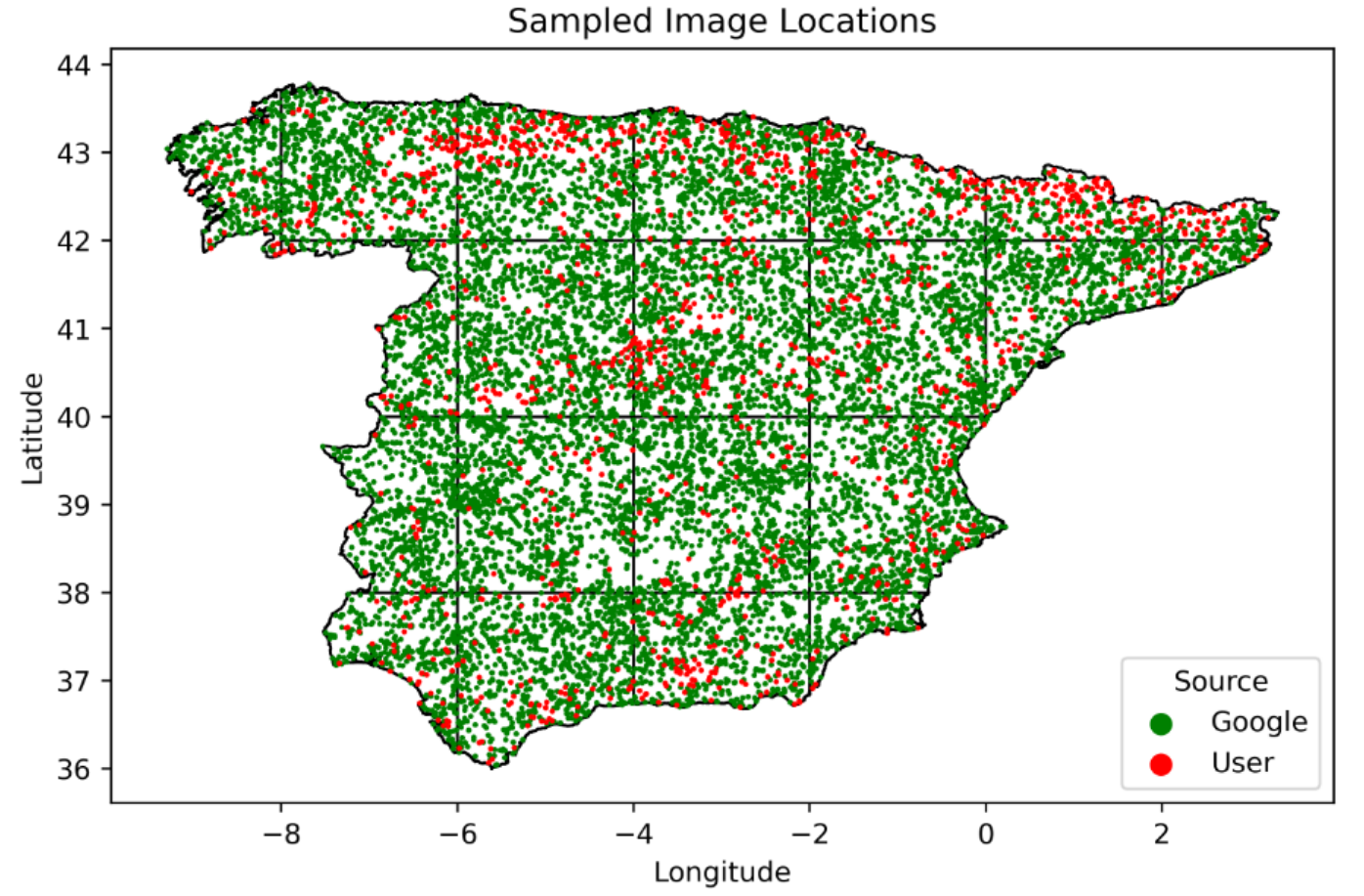
The project began with the collection of 13,099 RGB images of mainland Spain from the Google Street View Static API. Mainland Spain was divided into 21 grids, and 1000 images were randomly sampled from each full-size grid with a proportional amount of image sampled from smaller grids based on their relative area. Each of the sampled images had size 600x600x3 and contained a copyright signature in the bottom right corner. If the photograph was taken by an official Google Street View vehicle equipped with a 3-D camera, the copyright signature simply reads ”Google.” However, the data set also contains images taken by regular people who upload the photos onto the Internet - these are marked with the photographer’s name rather than ”Google.” With this convenient signature, I was able to classify the source of all 13,099 images as being the Google Street View vehicle or not. With the input data fully prepared at this point, the calculation of feature descriptors could begin.

Location of 13,099 images sampled from Google Street View API. Point color represents whether the image was taken by the Google Street View vehicle or a user who uploaded the image online.

Feature Calculation

The next step was to calculate the feature descriptors that were found to have some predictive value for geolocation in the original IM2GPS paper.¹ The feature descriptors used in the final model are listed below.

• Color histograms: Each 600x600x3 RGB input image was converted to the CIELAB color space, which contains three dimensions: L* (lightness), a* (green-red), and b* (blue-yellow). Then, each pixel of an image was placed into a 3D histogram where the L* axis held four bins while the a* and b* axes held 14 bins. The CIELAB color space is device-independent, meaning that the values used to produce a color will have the same output through any device. This characteristic is not shared by the RGB color space.⁵ Furthermore, the CIELAB color space is based upon the human perception of color, so it has held particular value in some computer vision applications.⁶

• Tiny images: Each 600x600x3 RGB input image was downscaled twice - once into a 16x16x3 RGB image, and again into a 5x5 CIELAB image. Despite their low resolution, past research has revealed that downscaled images maintain high recognizability while reducing computational expense.⁷

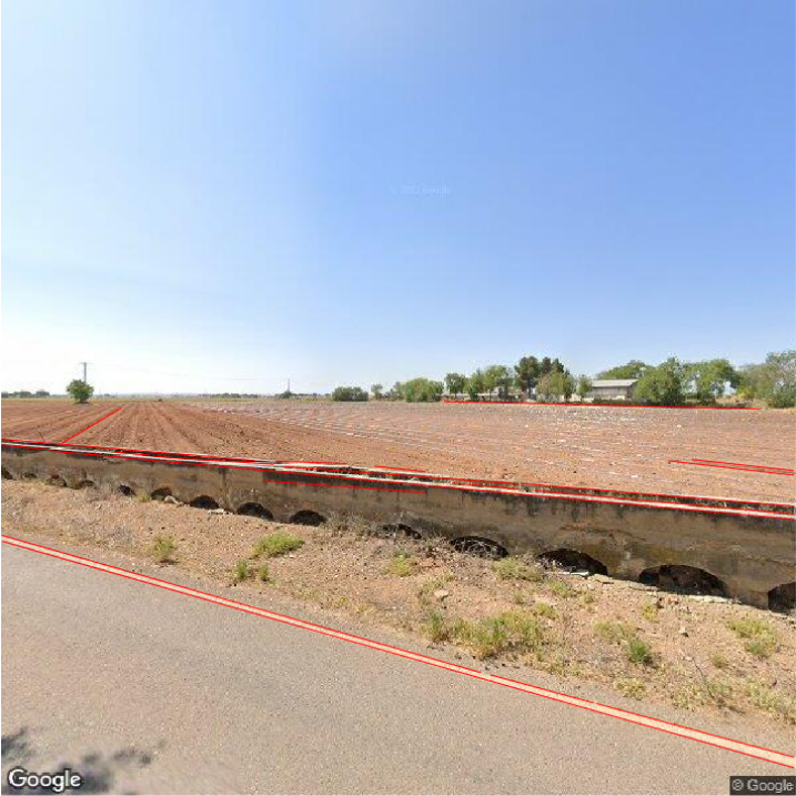
• Line features: Another feature of interest was the statistics pertaining to detected straight lines within the image. Straight lines were detected using the methodology presented in Video Compass.⁸ First, I identified edges in the grayscale version of an image with the Canny detector. Then, I found the connected components of the binary edge matrix and iterated through them. All connected components of length less than 5% of the image size were discarded. As described in Video Compass,⁸ the best fit line was computed for the remaining connected components and lines with satisfactory fit quality remained. Using the parameters of the best fit line for these connected components, I obtained line angle and length. After completing this process for all connected components within a single image, I computed histogram count vectors with 17 bins for both line angle and line length.

Example of straight line detection on an input image

• Texton histograms: Next, I calculated a histogram of textons for each image. Calculating this feature required the creation of a universal texton dictionary. First, I applied a filter bank (a steerable pyramid with four scales and two orientations) to four randomly selected images from each grid (the 21 grids dividing mainland Spain) of our image data set, thus providing 84 total training images. I collected he filter responses for each image, yielding a 360000x8 data matrix because each image has 360,000 pixels. With 84 training images and their individual data matrices concatenated, we obtain a 30240000x8 data matrix. Then, I applied K-means clustering to find 32 cluster centers within this data. Once the 32 cluster centers are obtained, I applied the filter bank to all 13,099 images in the data set and captured the 1x8 vector for each pixel representing the filter responses in each band of the steerable pyramid. I assigned each of these vectors to one of the 32 cluster centers, essentially yielding a 600x600 matrix of cluster labels for each image, which was then converted into a 1x32 vector representing texton histogram counts.

• Gist descriptor: The gist descriptor⁹ is a global feature descriptor that has been found to perform well in scene classification.¹ I calculated it for each image by applying a bank of Gabor filters with four scales and six orientations to each image, yielding 24 bands. I divided each of these patches into a 4x4 grid (16 grids of size 150x150 in the case of a 600x600 input image) and calculated the mean filter response in each cell. Completing this process for all 24 patches means that the total output for a single image is a vector of length 384, which we call the gist descriptor.

At this point, each input image had the following corresponding features calculated: a 16x16 RGB tiny image, 5x5 CIELAB tiny image, CIELAB color histogram, texton histogram, line feature histogram, and gist descriptor

Convolutional neural network with classical features

The final model takes in eight inputs:

• Image of shape 300x300x3 (original 600x600x3 image was downscaled due to memory limitations)
• Color histogram vector of length 784
• Gist descriptor vector of length 384
• Texton histogram vector of length 32
• Line angle vector of length 17
• Line length vector of length 17
• Tiny RGB image vector of length 768
• Tiny LAB image vector of length 75

Feature-based convolutional neural network

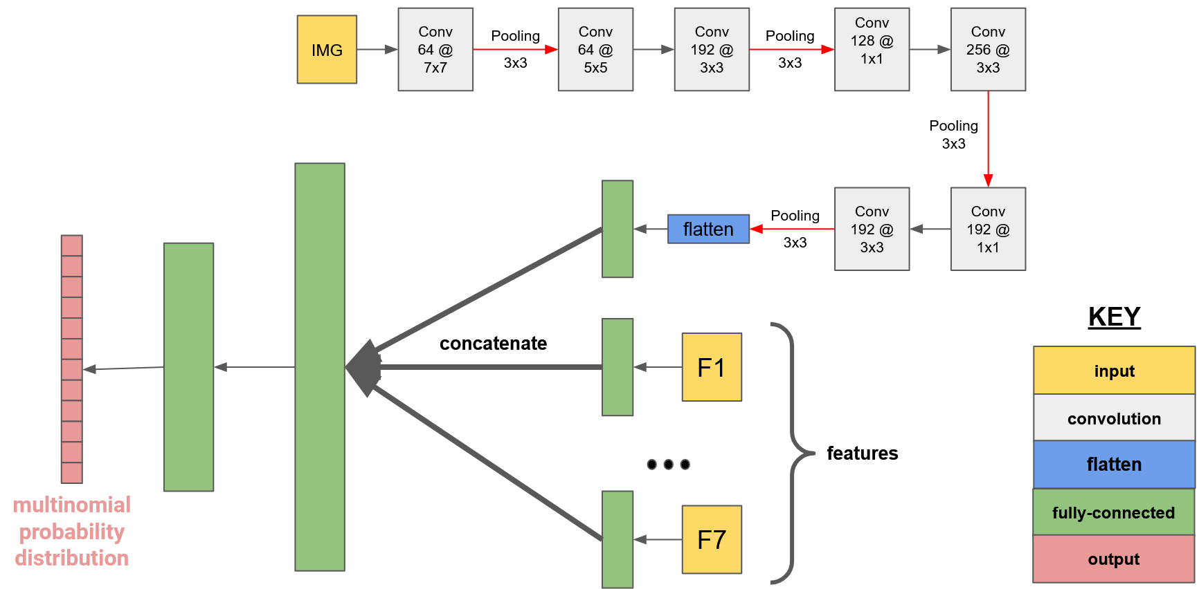
Notice that while the image takes the form of a matrix, each of the feature descriptor inputs have been flat- tened into vectors. This pre-processing flattening step is necessary because the non-image inputs are not passed into the convolution layers. Rather, they are only incorporated into the fully-connected stage of the neural network, at which point they must have a one-dimensional shape.

Each of the seven non-image inputs are passed into fully-connected layers and their outputs are concatenated to that of the image layer. With eight fully-connected layers consisting of 128 units, the concatenated layer has shape 1024. Similarly to the previous model, this output passes through final non-linear fully-connected layers until it outputs a multinomial probability distribution representing the predicted probability of the image being from each grid. A weighted average is computed on all 21 grid center points (weighted by each grid’s corresponding modeled probability), the output of which represents the model’s predicted geolocation.

Results

The map below is overlayed with all of the predicted image locations.

Map with predicted image locations

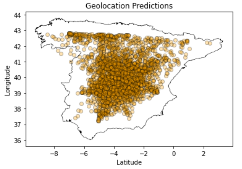
Note that the weighted average approach naturally makes “conservative” predictions towards the middle more likely. Predictions along the borders are impossible at most spots.

The final model’s performance metrics in comparison with a random “guessing” approach can be found below.

Metric	Random	Model
Accuracy	5.78%	16.56%
MAE	385.0	269.0
MSE	184658	96163
<200km	18.32%	39.54%

Accuracy refers to how often the correct grid is chosen (of 21 total choices). MAE and MSE refer to mean absolute error and mean squared error respectively. The “<200km” metric refers to how often the predicted geolocation is within 200 kilometers of the actual location - an arbitrary value chosen to represent “pretty good” predictions.

Distribution of prediction error along with a reference plot

Discussion

In summary, I implemented and analyzed three models (see paper for full details) for small-scale photo geolocation: a 1-NN approach utilizing classical features, a convolutional neural network taking in a single input image, and a convolutional neural network taking in an input image along with seven classical features as separate inputs.

I found that all of the models outperformed the approach of random predictions, but their respective performance varied. Specifically, the feature-based 1-NN approach exhibited the worst performance as both convolutional networks were massive improvements over the feature-based model.

A comparison between both CNN implementations reveals that the incorporation of feature descriptors did yield a slight improvement in performance. However, this increase in accuracy is not significant enough to confidently draw any conclusions and further analysis is necessary to confirm the value (or lack thereof) of classical features as secondary inputs into a convolutional neural network for photo geolocation. For the time being, the results suggest that classical features do not offer much value for photo geolocation when convolutional neural networks are an option.

It should be noted that even the optimized convolutional neural networks do not achieve accuracy anywhere near the level necessary to be used as a means for geotagging. A mean error of approximately 270 kilometers is still significant even if it’s a clear improvement over the random approach.

Attempting to use these models for precise geotagging would yield extremely misleading results and should thus be avoided. A more realistic use case would be to use modeled probability distributions as a prior for other computer vision tasks.

1. Hays, James, and Alexei A. Efros. ”IM2GPS: estimating geographic information from a single image.” Proceedings of the IEEE Conf. on Computer Vision and Pattern Recognition. IEEE, 2008. ↩ ↩² ↩³ ↩⁴ ↩⁵

2. Browning, Kellen. “Siberia or Japan? Expert Google Maps Players Can Tell at a Glimpse.” The New York Times, The New York Times, 7 July 2022, https://www.nytimes.com/2022/07/07/business/geoguessr-google-maps.html. ↩

3. Murgese, Fabio, et al. ”Automatic Outdoor Image Geolocation with Focal Modulation Networks.” (2022). ↩

4. Weyand, Tobias, Ilya Kostrikov, and James Philbin. ”Planet-photo geolocation with convolutional neural networks.” European Conference on Computer Vision. Springer, Cham, 2016. ↩

5. Kaur, Amanpreet, and B. V. Kranthi. ”Comparison between YCbCr color space and CIELab color space for skin color segmentation.” International Journal of Applied Information Systems 3.4 (2012): 30-33. ↩

6. Krieger, Louis WMM, et al. ”Method for improving skin color accuracy of three-dimensional printed training models for early pressure ulcer recognition.” Innovations and Emerging Technologies in Wound Care. Academic Press, 2020. 245-279. ↩

7. Torralba, Antonio, Rob Fergus, and William T. Freeman. ”Tiny images.” (2007). ↩

8. Kosecka, Jana, and Wei Zhang. ”Video compass.” European Conference on Computer Vision. Springer, Berlin, Heidelberg, 2002. ↩ ↩²

9. Oliva, Aude, and Antonio Torralba. ”Modeling the shape of the scene: A holistic representation of the spatial envelope.” International Journal of Computer Vision 42.3 (2001): 145-175. ↩